An Introduction to the dataset

The data set can be found here on Kaggle. It consists of 7 columns and 30758 rows. The data type of all columns are strings and contains no NULL values. The dataset does contain strings labeled as Nan, which are placeholders for np.nan.

Make sure you download the .csv file and move it to the working directory of your Jupyter Notebook.

Filtering and Pre-processing the data

Preprocessing data is always the first step in building any usable dataset. It helps eliminate all the unnecessary data that we won't be using. By preprocessing the data, we are essentially helping the program only look at relevant data.

Importing the Required Libraries

import matplotlib.pyplot as plt
import pandas as pd
import numpy as np
import seaborn as sns
from wordcloud import WordCloud

Loading data as a Pandas DataFrame

dataset = pd.read_csv('FashionDataset.csv')  # Importing CSV file
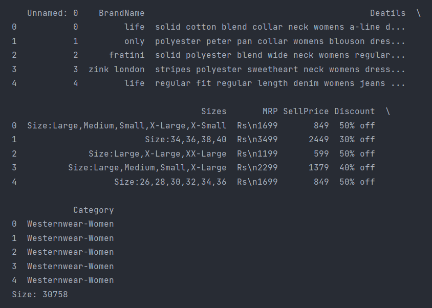
print(dataset.head())
print(f"Size: {dataset.shape[0]}")  # Number of Rows

Dropping Unnecessary Columns

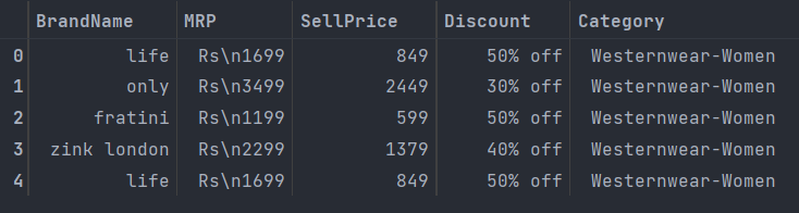
data_set_trim_1 = dataset.drop(['Deatils', "Sizes", 'Unnamed: 0'], axis=1)  # Since we only care about numeric data, for now, we can remove all the data we don't need (also, yes details is spelled like that in the dataset)
data_set_trim_1.head()

Output:

Pre-Processing the data

data_set_trim_1["MRP"] = data_set_trim_1["MRP"].str.replace("Rs\n", "")  # 'Rs\n420' -> '420'
data_set_trim_1["Category"] = data_set_trim_1["Category"].str.replace("-Women", "")  # 'Watch-Women' -> 'Watch'
data_set_trim_1["Discount"] = data_set_trim_1["Discount"].str.replace("% off", "")  # '50% off' -> '50'
data_set_trim_1.head()

Output:

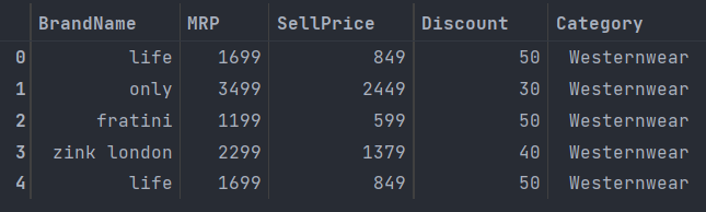
At this point, I thought the data would be converted to integers, but I was wrong all the data were still strings. To verify this, I ran the following one-liner

type(data_set_trim_1.iloc[22]["SellPrice"])  #Noticing that SellPrice as well as MRP and Discount are Strings and not text

Output:

str

Now I would convert all the strings into integers using the .apply() attribute and replace the string Nan values with actual np.NaN values

data_set_trim_2 = data_set_trim_1.replace("Nan",np.nan)  # Replacing all "Nan" strings with np.NAN
data_set_trim_2.dropna(inplace=True, subset=['MRP', "BrandName", "SellPrice"])
print(data_set_trim_2.dtypes)  # All Columns are String DataType
data_set_trim_2[['MRP', 'SellPrice', "Discount"]] = data_set_trim_2[['MRP', 'SellPrice', "Discount"]].apply(pd.to_numeric)  # Changing Required Columns to integer
print(data_set_trim_2.dtypes)

Output

BrandName    object
MRP          object
SellPrice    object
Discount     object
Category     object
dtype: object
BrandName    object
MRP           int64
SellPrice     int64
Discount      int64
Category     object
dtype: object

Finalising the data

f_data = data_set_trim_2  # Setting Final Data
print(f"Size: {f_data.shape[0]}")

we return with 22550 rows worth of complete data. Now we can start visualizing it ;)

Accessing Basic Information

Let's start with something Simple. How many unique brands do we have in our dataset?

f_data.nunique()["BrandName"]  # Number of Brands in Dataset

Output:

That's a lot of brands! Let's get a deeper look at the data using the .describe() command

f_data.describe().T

Output:

What about the most expensive Items?

f_data[f_data.SellPrice == f_data.SellPrice.max()]  # Most Expensive Item(s)

Output:

(Yikes! Those are some expensive watches)

What about the most expensive brands? Let's figure out the average price of any article from a brand

f_data.groupby('BrandName')['SellPrice'].mean().sort_values(ascending=False).head()  # Mean Price of every Brand

Output:

BrandName
just cavalli      18309.600000
coach             12616.769231
versus            11555.600000
ted baker         10031.111111
emporio armani     9423.509804
Name: SellPrice, dtype: float64

You can similarly find the cheapest brand by changing ascending=False to True

Real Visualizations using Matplotlib and Seaborn

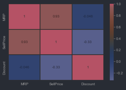
Let's start by plotting a heatmap of our data.

sns.heatmap(f_data.corr(),annot=True,cmap='coolwarm',linewidths=0.2)

Output:

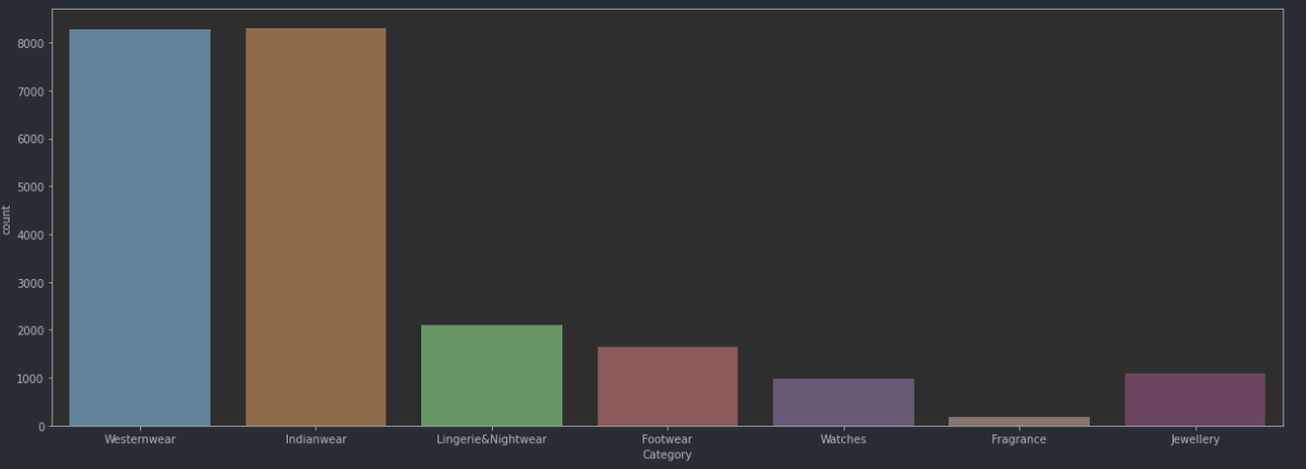
What about a plot which shows us the amount of items in each category?

plt.figure(figsize=(20,7))  #setting the plot size
sns.countplot(f_data["Category"])

Output:

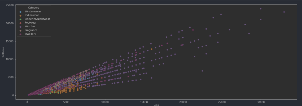
Here is a scatter plot of all the prices per category

plt.figure(figsize=(20,7))
sns.scatterplot(f_data['MRP'],f_data['SellPrice'],hue=f_data['Category'])

Output:

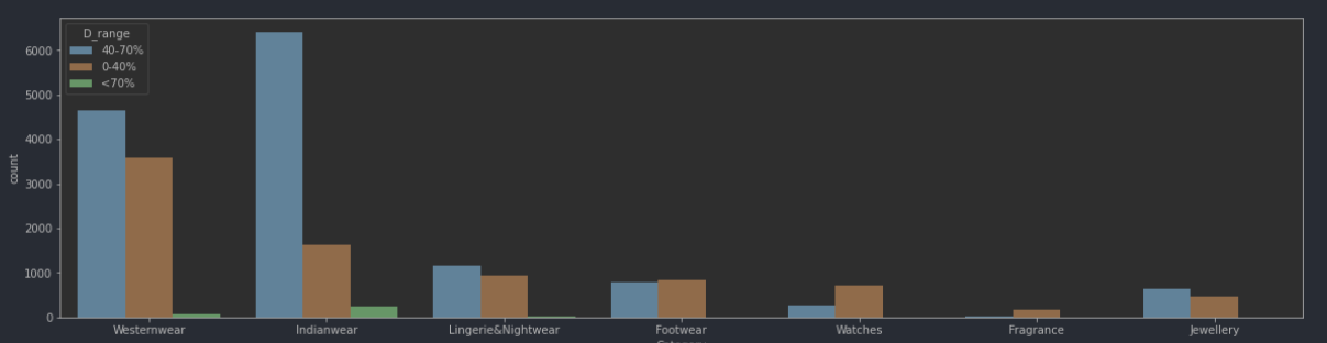
Let's figure out which category is the most discounted

def modify(d):
    if int(d) in range(0,41):
        return '0-40%'
    elif int(d) in range(41,71):
        return '40-70%'
    elif int(d) in range(71,101):
        return '<70%'
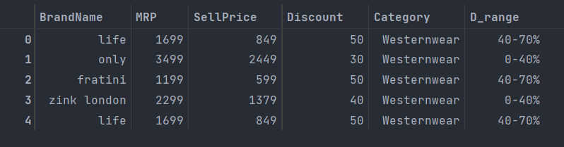
f_data['D_range'] = f_data['Discount'].apply(modify)  # adding a new column
f_data.head()

plt.figure(figsize=(20,5))
sns.countplot(f_data['Category'],hue=f_data['D_range'])

Output:

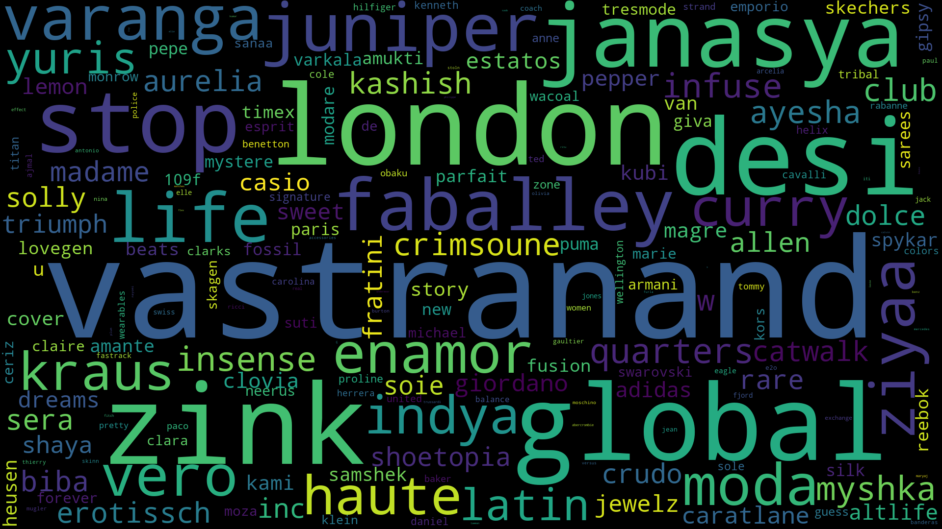
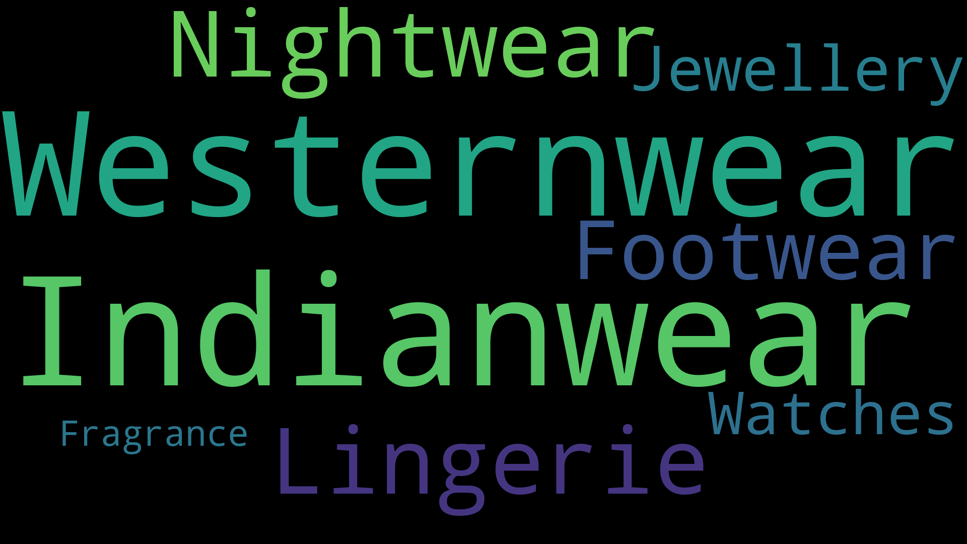
Fun with WordClouds

We've had some interesting plots, but now let's have some fun with '✨word clouds✨

Since the Word Cloud Module takes a string as input we are going to be joining the various strings

textCategory = " ".join(i for i in f_data['Category'])
textCompany = " ".join(i for i in f_data['BrandName'])

word_cloud_company = WordCloud(collocations=False, background_color='black', width=1920, height=1080).generate(textCompany)
word_cloud_company.to_file('company.png')

word_cloud_category = WordCloud(collocations=False, background_color='black', width=1920, height=1080).generate(textCategory)
word_cloud_category.to_file('category.png')

Output:

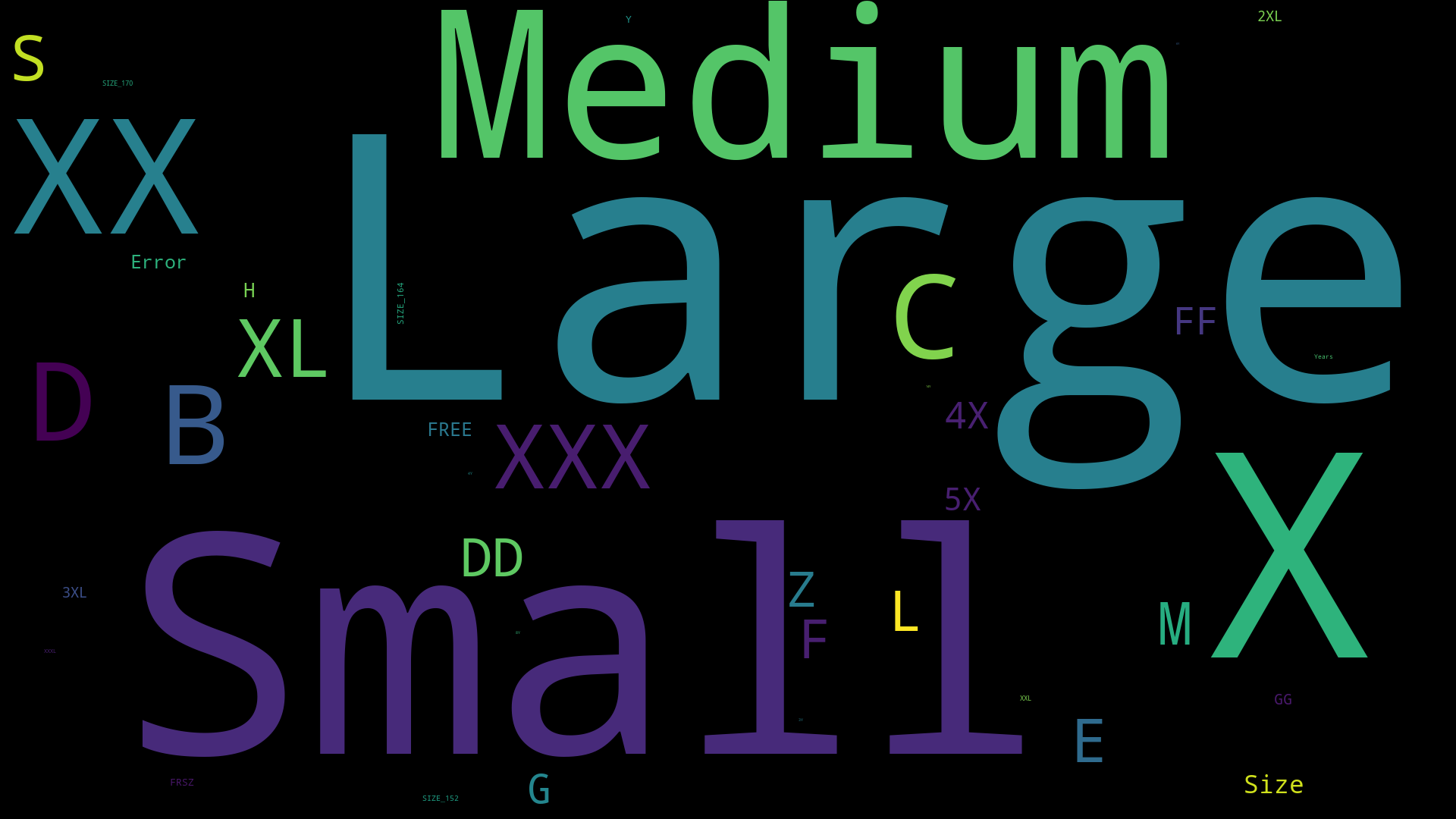
How about using the sizes column we dropped while preprocessing

Let's make a word cloud of the Sizes and Details column!

#Processing the data

only_size = dataset["Sizes"]
only_size = only_size.replace("Nan",np.nan)  # Replacing all "Nan" strings with np.NAN
only_size.dropna(inplace=True)
only_size = only_size.str.replace("Size:", "")
only_size = only_size.str.replace(",", " ")
only_size.head()

textSize = " ".join(i for i in only_size)
word_cloud_size = WordCloud(collocations=False, background_color='black', width=1920, height=1080).generate(textSize)
word_cloud_size.to_file('size.png')

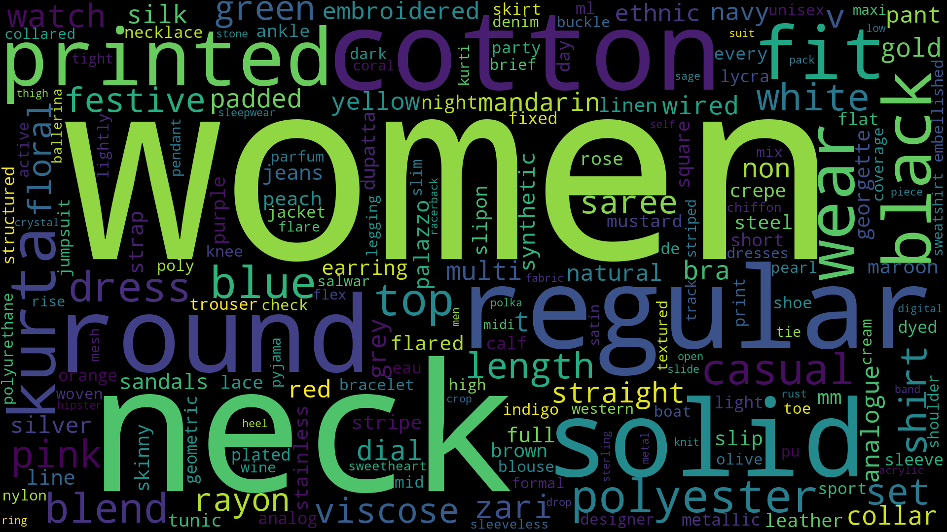
Similarily we can do the same thing with the details column

only_details = dataset["Deatils"]
only_details = only_details.replace("Nan",np.nan)  # Replacing all "Nan" strings with np.NAN
only_details.dropna(inplace=True)
only_details = only_details.str.replace("Size:", "")
only_details = only_details.str.replace(",", " ")
only_details.head()

textDetail = " ".join(i for i in only_details)
word_cloud_detail = WordCloud(collocations=False, background_color='black', width=1920, height=1080).generate(textDetail)
word_cloud_detail.to_file('detail.png')

Conclusion

Well, that's all, folks! I don't really have a conclusion, but DATA IS SO COOL!

You can find the Google Colab Link here

Visualizing Data — Women's Fashion Catalog

Comments

✨Visualizing Data✨

Penalties and The World Cup ⚽

More from this blog

LLM Classifiers: Don't Just Classify, Conquer

Friendship over with Attention. Now FNet is my best friend

PaliGemma 2 - VLMs made easy

An honest Guide to Optimize LLMs for upto 10x Inference

My Journey as a Developer - DevRetro 2023

An Introduction to the dataset

Filtering and Pre-processing the data

Importing the Required Libraries

Loading data as a Pandas DataFrame

Dropping Unnecessary Columns

Pre-Processing the data

Finalising the data

Accessing Basic Information

Real Visualizations using Matplotlib and Seaborn

Fun with WordClouds

Conclusion

Command Palette

Comments

✨Visualizing Data✨

Penalties and The World Cup ⚽

More from this blog

An Introduction to the dataset

Filtering and Pre-processing the data

Importing the Required Libraries

Loading data as a Pandas DataFrame

Dropping Unnecessary Columns

Pre-Processing the data

Finalising the data

Accessing Basic Information

Real Visualizations using Matplotlib and Seaborn

Fun with WordClouds

Conclusion